The city of Austin has a very nice Open Data Portal. After digging a little bit I found that the most popular datasets in the portal are related to dogs, which it is not a surprise, since we are talking about the city of Austin. The truth is that there is a lot of data available. For this example, I’m going to be using the City of Austin Employee Detail Information for two reasons. One, it’s always interesting to see salaries and two, because I can try to reproduce the analysis that the people from the Texas Tribune are doing with the same data set.

Getting started

Obviously, I’m going to be using Python with Anaconda. You can find the installer and the instructions at the Continuum Analytics’s website. Once Anaconda has been installed, we are ready to go, since all the libraries are already part of the distribution.

We will start by importing pandas, numpy and matplotlib:

import pandas as pd
import numpy as np
import matplotlib.pyplot as plt

Then we will load the CSV file into pandas. Since the column Annual Salary has a data type of dtype('O'), we will need to convert into a float. As you can imagine, the problem is the $ sign:

df = pd.read_csv('City_of_Austin_Employee_Detail_Information.csv')
df[['Emp ID', 'Last', 'Annual Salary']][0:10]

| index  | Emp ID   | Last            | Annual Salary |
|--------|----------|-----------------|---------------|
| 0      | 10000003 | Turner          | $62608.00     |
| 1      | 10000008 | Michael         | $146101.28    |
| 2      | 10000015 | Greco           | $96345.60     |
| 3      | 10000022 | Wiswell-DeCampo | $45676.80     |
| 4      | 10000026 | White           | $109867.68    |
| 5      | 10000039 | Candoli         | $100800.96    |
| 6      | 10000066 | Mason           | $126349.60    |
| 7      | 10000084 | Lynch           | $94203.20     |
| 8      | 10000127 | Wosky           | $93977.52     |
| 9      | 10000132 | Ringuette       | $75487.36     |

We will create a new column called annual_salary with a parsed value from Annual Salary, so we can play with the data from this column.

df['annual_salary'] = df['Annual Salary'].map(lambda x: float(x.strip('$')))

Interesting findings

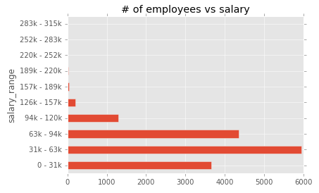
Most of the employees (28%) earns between 31k - 63k:

33% of males employees earn between 63k and 94k, against only 18% of female employees.

df[df['Gender'] == 'M'].groupby('salary_range')['Gender'].count()[2]/len(df[df['Gender'] == 'M'])
# => 0.33009231978000392
df[df['Gender'] == 'F'].groupby('salary_range')['Gender'].count()[2]/len(df[df['Gender'] == 'F'])
# => 0.18786289567334707

There is more people working in Parks & Recreation (2362) than in the police (2358).

Finally it’s pretty clear that most of the employees are white:

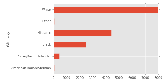
The rest of the analysis is nothing but pandas standard and you can check the jupyter notebook here. You can also play with it using Binder here (find it under the notebooks directory).